5. Spike-in analysis (human)#
Here we show the spike-in analysis using Churros. Spike-in analysis is a method to normalize the ChIP-seq data by adding a known amount of external DNA as an internal control. This method allows us to compare ChIP-seq samples at an absolute level.
In this tutorial, we will use the ChIP-seq data of H3K79me2 histone modification data for Jurkat cells from Orlando et al., Cell Reports, 2014. The sample scripts are also available at Churros GitHub site.
H3K79me2 modification is lost from chromatin by treatment with the DOT1L inhibitor EPZ5676. In this experiment, EPZ5676-treated cells (low H3K79me2 levels) were mixed with DMSO-treated cells (high H3K79me2 levels) at ratios of 0%, 25%, 50%, 75%, and 100%. Therefore, in the ChIP-seq data, the higher the proportion of EPZ5676-treated cells, the lower the enrichment of H3K79me2 peaks should be.
Note
churros.sif). Please add apptainer exec churros.sif before each command below.apptainer exec churros.sif download_genomedata.sh5.1. Get data#
Here we use pfastq-dump to download the fastq files from the SRA database.
mkdir -p fastq
for id in SRR1536557 SRR1536558 SRR1536559 SRR1536560 SRR1536561 SRR1584489 SRR1584490 SRR1584491 SRR1584492 SRR1584493
do
    pfastq-dump -s $id -t 4 --outdir fastq/ --gzip
done
Then download and generate the reference dataset including genome, gene annotation and index files.
The reference genome is human, while the spike-in DNA is the D. melanogaster.
Here we specify hg38 and dm6 for genome build.
mkdir -p log
ncore=24
for build in hg38 dm6
do
    Ddir=Referencedata_$build
    download_genomedata.sh -s $build $Ddir 2>&1 | tee log/$Ddir
    build-index.sh -p $ncore bowtie2 $Ddir
done
5.2. Prepare sample list#
The format of samplelist.txt and samplepairlist.txt is the same with the normal analysis.
5.2.1. samplelist.txt#
H3K79me2_0_rep1 fastq/SRR1536557.fastq.gz
H3K79me2_25_rep1        fastq/SRR1536558.fastq.gz
H3K79me2_50_rep1        fastq/SRR1536559.fastq.gz
H3K79me2_75_rep1        fastq/SRR1536560.fastq.gz
H3K79me2_100_rep1       fastq/SRR1536561.fastq.gz
WCE_0_rep1      fastq/SRR1584489.fastq.gz
WCE_25_rep1     fastq/SRR1584490.fastq.gz
WCE_50_rep1     fastq/SRR1584491.fastq.gz
WCE_75_rep1     fastq/SRR1584492.fastq.gz
WCE_100_rep1    fastq/SRR1584493.fastq.gz
5.2.2. samplepairlist.txt#
H3K79me2_0_rep1,WCE_0_rep1,H3K79me2_0_rep1,sharp
H3K79me2_25_rep1,WCE_25_rep1,H3K79me2_25_rep1,sharp
H3K79me2_50_rep1,WCE_50_rep1,H3K79me2_50_rep1,sharp
H3K79me2_75_rep1,WCE_75_rep1,H3K79me2_75_rep1,sharp
H3K79me2_100_rep1,WCE_100_rep1,H3K79me2_100_rep1,sharp
5.3. Running Churros#
The churros command has a --spikein option to run in spike-in mode.
In spike-in mode, in addition to the normal arguments, the genome build and the reference data directory of the spike-in genome should be specified by the --build_spikein and --Ddir_spikein options, respectively.
ncore=48
build=hg38
build_spikein=dm6
Ddir_ref=Referencedata_$build
Ddir_spikein=Referencedata_$build_spikein

churros -p $ncore --spikein samplelist.txt samplepairlist.txt \
    $build $Ddir_ref --build_spikein $build_spikein --Ddir_spikein $Ddir_spikein
The output directory contains several new subdirectories:
dm6/: Map files mapped to the spike-in genome. The directory name depends on the genome build. In this case it isdm6/.bigWig/Spikein/: bigWig files that have been spike-in normalized. Use these files for downstream analysis.pdf_spikein/: Visualization files that have been spike-in normalized. Thepdf/directory contains visualization files with total read normalization as usual.spikein_scalingfactor/: A scaling factor calculated from the number of reads in the spike-in genome. Reads are normalized to this value.
Note
Currently, spike-in normalization is not applied to peak calling with MACS3.
Let’s look at the read distribution with total read normalization (in the pdf/ directory) and spike-in normalization (in the pdf_spikein/ directory). The first page of chromosome 10 (drompa+.bin5M.PCSHARP.5000_chr10.pdf) looks like this.
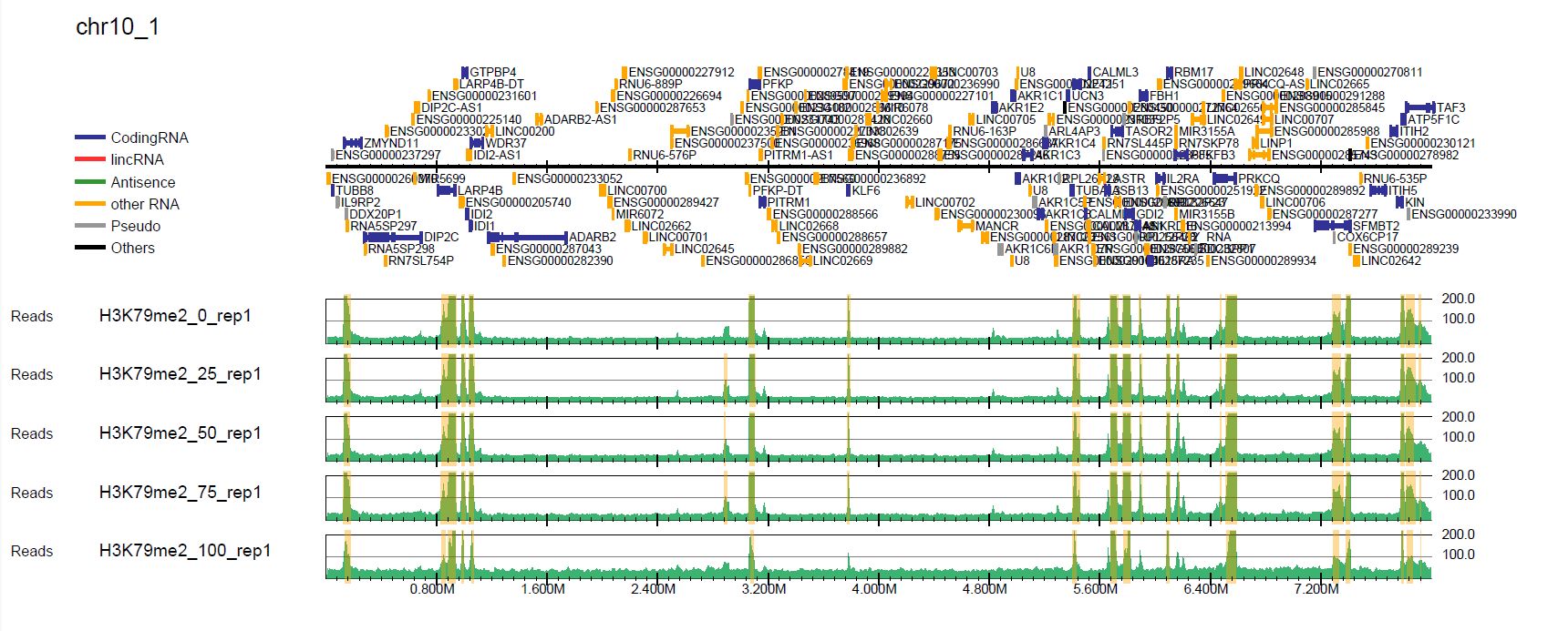
Fig. 5.1 Total read normalization#
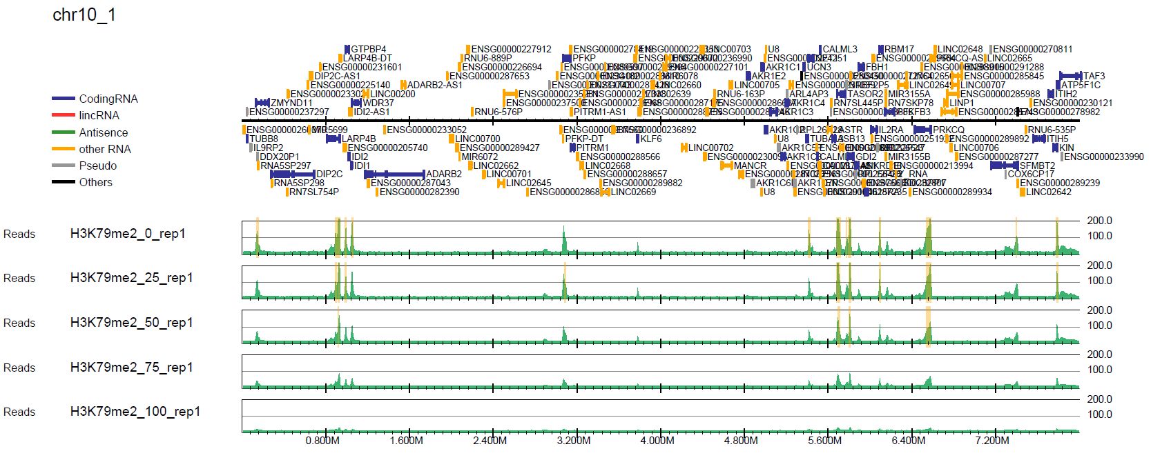
Fig. 5.2 Spike-in normalization#
In the spike-in normalization, we can see the decreased enrichment of H3K79me2, while the total read normalization does not successfully show it.
5.3.1. Generate a read distribution profile#
With the generated bigWig files, you can perform downstream analysis such as plotting the averaged profile. Churros uses DROMPAplus internally, which has a command to generate a read distribution profile in the PDF format. You can use it to see the averaged read distribution for spike-in normalization.
The command for DROMPAplus is as follows. See the DROMPAplus manual for details.
build=hg38
Ddir_ref=Referencedata_${build}
gt=$Ddir_ref/genometable.txt
gene=$Ddir_ref/gtf_chrUCSC/chr.proteincoding.gene.refFlat

mkdir -p profile

pdir=Churros_result_Quickstart/hg38/bigWig/TotalReadNormalized
s1="-i $pdir/H3K79me2_0_rep1.100.bw,$pdir/WCE_0_rep1.100.bw,H3K79me2_0_rep1"
s2="-i $pdir/H3K79me2_25_rep1.100.bw,$pdir/WCE_25_rep1.100.bw,H3K79me2_25_rep1"
s3="-i $pdir/H3K79me2_50_rep1.100.bw,$pdir/WCE_50_rep1.100.bw,H3K79me2_50_rep1"
s4="-i $pdir/H3K79me2_75_rep1.100.bw,$pdir/WCE_75_rep1.100.bw,H3K79me2_75_rep1"
s5="-i $pdir/H3K79me2_100_rep1.100.bw,$pdir/WCE_100_rep1.100.bw,H3K79me2_100_rep1"

$sing drompa+ PROFILE --gt $gt -g $gene $s1 $s2 $s3 $s4 $s5 -o profile/TotalReadNormalized-H3K79me2 --widthfromcenter 10000

pdir=Churros_result_Quickstart/hg38/bigWig/Spikein
idir=Churros_result_Quickstart/hg38/bigWig/RawCount
s1="-i $pdir/H3K79me2_0_rep1.100.bw,$idir/WCE_0_rep1.100.bw,H3K79me2_0_rep1"
s2="-i $pdir/H3K79me2_25_rep1.100.bw,$idir/WCE_25_rep1.100.bw,H3K79me2_25_rep1"
s3="-i $pdir/H3K79me2_50_rep1.100.bw,$idir/WCE_50_rep1.100.bw,H3K79me2_50_rep1"
s4="-i $pdir/H3K79me2_75_rep1.100.bw,$idir/WCE_75_rep1.100.bw,H3K79me2_75_rep1"
s5="-i $pdir/H3K79me2_100_rep1.100.bw,$idir/WCE_100_rep1.100.bw,H3K79me2_100_rep1"

$sing drompa+ PROFILE --gt $gt -g $gene $s1 $s2 $s3 $s4 $s5 -o profile/Spikein-H3K79me2 --widthfromcenter 10000
The results are in the profile/ directory.
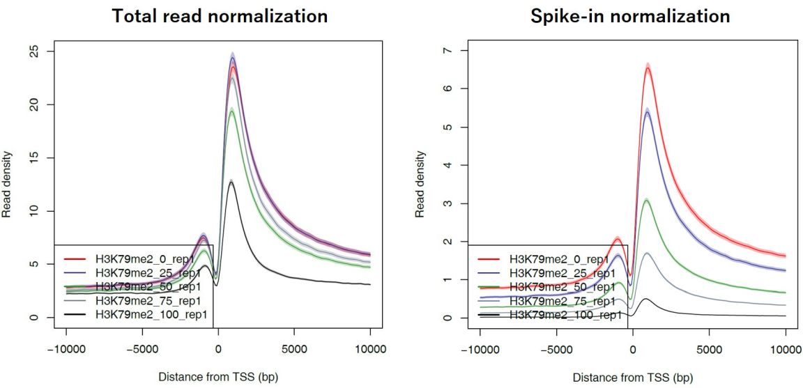
Fig. 5.3 Averaged read distribution around TSSs of all protein-coding genes#
5.4. Execute a single step#
5.4.1. churros_mapping_spikein#
If you just want to do the mapping and generate bigWig files for spike-in normalization, use the churros_mapping_spikein command.
build=hg38
build_spikein=dm6
Ddir_ref=Referencedata_${build}
Ddir_spikein=Referencedata_${build_spikein}
ncore=48

churros_mapping_spikein exec samplelist.txt samplepairlist.txt -p ${ncore} \
    ${build} ${build_spikein} \
    ${Ddir_ref} ${Ddir_spikein}
5.4.2. churros_visualize#
If you want to generate PDF files for spike-in normalization, supply the options to churros_visualize as follows.
build=hg38
Ddir=Referencedata_$build
# Spike-in normalization (in the pdf_spikein directory)
churros_visualize --pdfdir pdf_spikein \
                  --chipdirectory Spikein --inputdirectory TotalReadNormalized \
                  samplepairlist.txt drompa+ $build $Ddir