4. Large-scale profile analysis

Churros provides a classheat function for clustering and visualizing large-scale epigenomic profiles. This function takes regions of interest (e.g., specific protein binding sites) as input 1 and a folder of epigenomic signal files (either binary or continuous) as input 2.

• In the binary mode, classheat outputs a binary matrix (output 1) representing the overlap of epigenomic markers at given genomic regions. The binary matrix is then formatted and sorted by the user-defined column (i.e., the filename of the selected marker) to generate the processed matrix (output 2) and plot the sorted heatmap (output 3). Subsequently, classheat utilizes PCA followed by k-means clustering (or other clustering methods) to produce the clustered matrix (output 4) and the clustered heatmap (output 5).

• In the continuous mode, classheat calculates the averaged read density of each epigenomic marker at given genomic regions (output 1). After logarithmic transformation, z-score normalization (optional method is 0-to-1 scaling), and sorting, classheat generates the remaining outputs in the same manner as in binary mode.

The main usages are:

churros_classheat mode region directory \
  [-k kcluster] [-s sortname] [-l samplelabel] [-n normalize type] [-m cluster method]

The required parameters:

• mode: either binary or continuous.

• region: a BED format file for regions of interest (input 1). Only the first 3 columns are used.

• directory: a directory containing the epigenomic signal files. The signal files can be either binary (e.g., peak files in BED format) or continuous (e.g., read coverage in bigwig format).

The optional parameters:

• -k kcluster: number of clusters for clustered matrix and clustered heatmap. The default value is 3.

• -s sortname: the filename of the selected marker in the directory above. This is used to for the processed matrix and sorted heatmap.

• -l samplelabel: A .tsv table used to assign groups for each marker in the directory above. For example, it could look like this.

H3K27ac_ENCSR000EWR_rep1_peaks.narrowPeak	H3K27ac
GATA3_ENCSR000EWV_rep1_peaks.narrowPeak	TFs
H3K9me3_ENCSR000EWQ_rep3.mpbl.100.bw	Histone
Rad21_ENCSR000BTQ_rep1_peaks.narrowPeak	TFs
…	…

• -n normalize type: Normalization methods for continuous data, could be zscore or scale0to1. Default: zscore.

• -m clustering method: minikmeans, kmeans, spectral, meanshift, dbscan, affinity

4.1. Example usage of binary mode

churros_classheat -l samplelabel.tsv binary Rad21_ENCSR000BTQ_rep1_peaks.narrowPeak ./peakdir/

This command takes as input a file representing regions of interest (Rad21_ENCSR000BTQ_rep1_peaks.narrowPeak) and a directory (./peakdir/) containing multiple epigenomic signals. We also assigned labels to the files in the ./peakdir/ directory. Five output files are generated:

Output1_raw_matrix.tsv
Output2_sorted_matrix.tsv
Output3_sorted_heatmap.png
Output4_kmeans_matrix.tsv
Output5_kmeans_heatmap.png

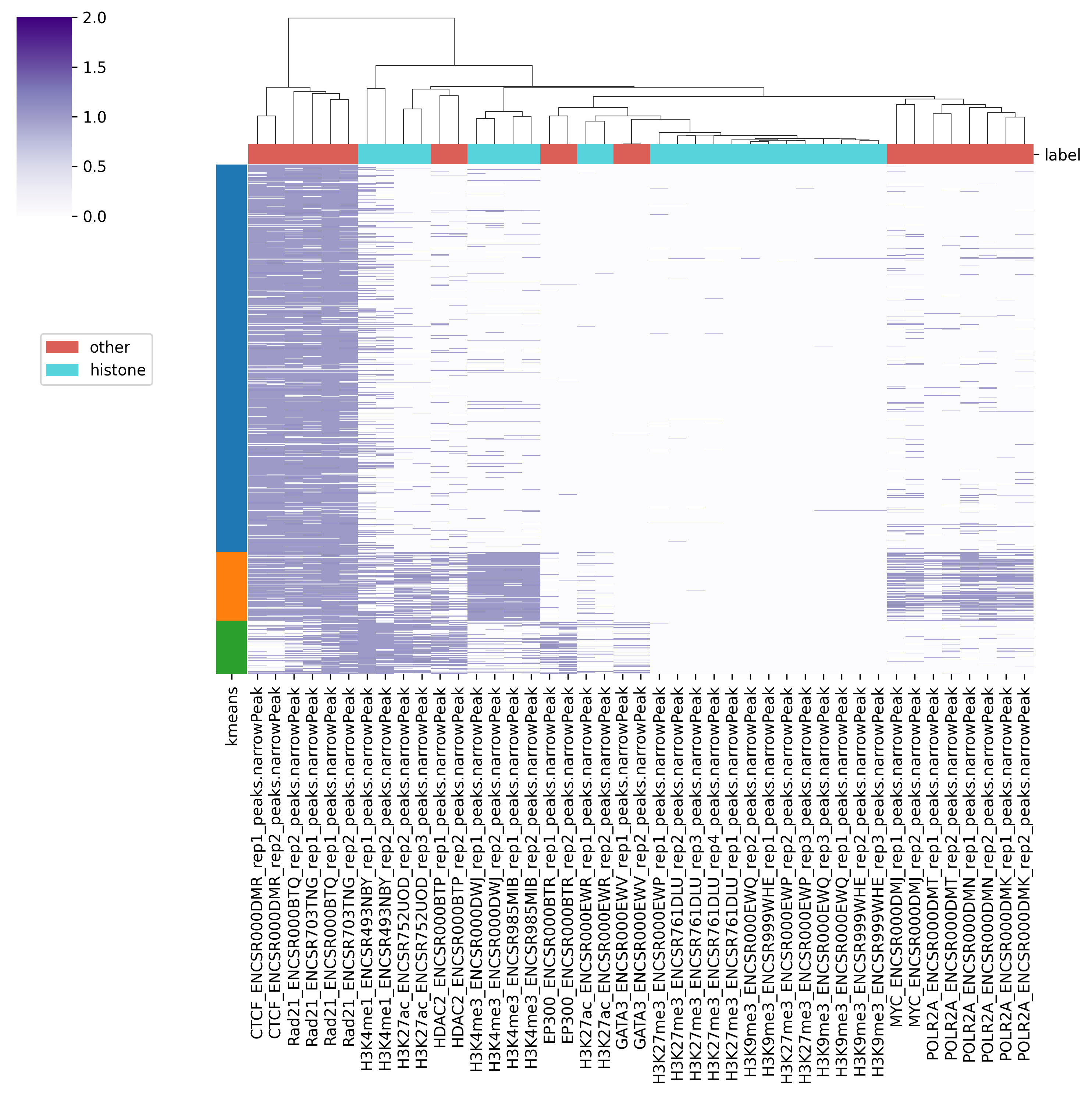
Fig. 4.1 Output5_kmeans_heatmap.png

4.2. Example usage of continuous mode

churros_classheat -l samplelabel.tsv -s GATA3_ENCSR000EWV_rep1.bw -k 3 -n zscore continuous Rad21_ENCSR000BTQ_rep1_peaks.narrowPeak ./bwdir/