6. Peakheatmap: Large-scale profile analysis#
Churros provides commands for clustering and visualizing large-scale peak profiles. These functions take a reference region (BED format) and cluster regions based on the overlap pattern of peaks or bigWig profiles. The sample scripts are also available at Churros GitHub site.
6.1. peakheatmap_binary: Binary comparison#
peakheatmap_binary outputs a binary matrix (output 1) representing the peak overlap for given genomic regions. The binary matrix is then formatted and sorted by the user-defined column (i.e., the filename of the selected marker) to generate the processed matrix (output 2) and plot the sorted heatmap (output 3). It then utilizes PCA followed by k-means clustering (or other clustering methods) to produce the clustered matrix (output 4) and the clustered heatmap (output 5).
The main usages are:
peakheatmap_binary <region> <directory>
The required parameters:
region: a BED file for regions of interest. Only the first 3 columns are used.
directory: a directory containing the peak files.
The optional parameters:
-k kcluster: number of clusters for clustered matrix and clustered heatmap. The default value is 3.
-s sortname: the filename of the selected marker in the directory above. This is used for the processed matrix and sorted heatmap.
-n normalize type: Normalization methods for continuous data, could be zscore or scale0to1. Default: zscore.
-m clustering method: minikmeans, kmeans, spectral, meanshift, dbscan, affinity
-l samplelabel: A .tsv table used to assign groups for each marker in the directory above. For example, it could look like this.
GATA3_ENCSR000EWV_rep1_peaks.narrowPeak protein
GATA3_ENCSR000EWV_rep2_peaks.narrowPeak protein
H3K27ac_ENCSR000EWR_rep1_peaks.narrowPeak       histone
H3K27ac_ENCSR000EWR_rep2_peaks.narrowPeak       histone
H3K27ac_ENCSR752UOD_rep2_peaks.narrowPeak       histone
H3K27ac_ENCSR752UOD_rep3_peaks.narrowPeak       histone
6.1.1. Example usage#
peakheatmap_binary -l samplelabel.tsv reference.bed ./peakdir/
This command takes as input a file representing regions of interest (reference.bed) and a peak directory (./peakdir/).
We also assigned labels to the files in the ./peakdir/ directory.
Five output files are generated:
Output1_raw_matrix.tsv
Output2_sorted_matrix.tsv
Output3_sorted_heatmap.png
Output4_kmeans_matrix.tsv
Output5_kmeans_heatmap.png
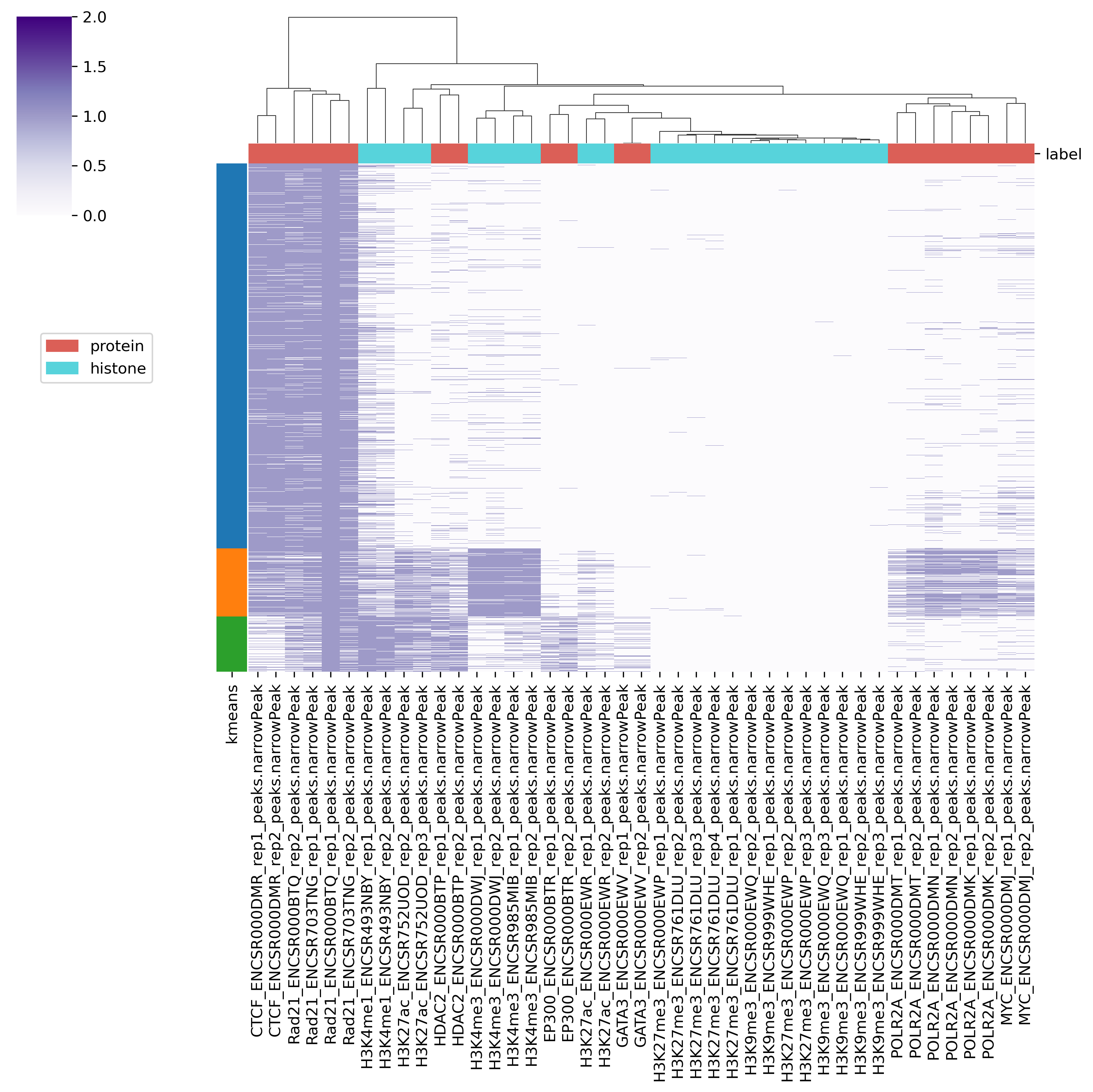
Fig. 6.1 Output5_kmeans_heatmap.png#
6.2. peakheatmap_quantitative: Quantitative comparison#
peakheatmap_quantitative calculates the read density of each ChIP samples at given genomic regions.
After log transformation, z-score normalization (optional method is 0-to-1 scaling), and sorting, it generates the remaining outputs in the same manner as in binary mode.
peakheatmap_quantitative [Options] <genometable> <region> <bigwigs>
   <genometable>: genome table file (e.g., genometable.txt)
   <region>: BED file of regions to analyze
   <bigwigs>: bigWig files for comparison (should be quoted)
   Options:
      -k <int>: number of clusters (default: 3)
      -b <int>: bin size (default: 1000)
      -s <str>: sort name (default: "defaultUseFirstColumn")
      -n <str>: normalization type (default: "zscore")
      -l <str>: sample label TSV file
      -m <str>: clustering method (default: "minikmeans")
      -o <str>: output directory (default: "output_quantitative/")
6.2.1. Example usage#
bwdir="Churros_result/hg38/bigWig/TotalReadNormalized/""
bws=`ls $bwdir/*.100.bw`

peakheatmap_quantitative -b 1000 genometable.txt reference.bed "$bws"